Intuition for the central limit theorem

Why the √n instead of n? What’s this weird version of an average?

If you have a bunch of perpendicular vectors \(x_1, \dotsc, x_n\) of length \(\ell\), then \(\frac{x_1 + \dotsb + x_n}{\sqrt{n}}\) is again of length \(\ell.\) You have to normalize by \(\sqrt{n}\) to keep the sum at the same scale.

There is a deep connection between independent random variables and orthogonal vectors. When random variables are independent, that basically means that they are orthogonal vectors in a vector space of functions.

(The function space I refer to is \(L^2\), and the variance of a random variable \(X\) is just \(\|X - \mu\|_{L^2}^2\). So no wonder the variance is additive over independent random variables. Just like \(\|x + y\|^2 = \|x\|^2 + \|y\|^2\) when \(x \perp y\).)¹

Why the normal distribution?

One thing that really confused me for a while, and which I think lies at the heart of the matter, is the following question:

Why is it that the sum \(\frac{X_1 + \dotsb + X_n}{\sqrt{n}}\) (\(n\) large) doesn’t care anything about the \(X_i\) except their mean and their variance? (Moments 1 and 2.)

This is similar to the law of large numbers phenomenon:

\(\frac{X_1 + \dotsb + X_n}{n}\) (\(n\) large) only cares about moment 1 (the mean).

(Both of these have their hypotheses that I’m suppressing (see the footnote), but the most important thing, of course, is that the \(X_i\) be independent.)

A more elucidating way to express this phenomenon is: in the sum \(\frac{X_1 + \dotsb + X_n}{\sqrt{n}}\), I can replace any or all of the \(X_i\) with some other RV’s, mixing and matching between all kinds of various distributions, as long as they have the same first and second moments. And it won’t matter as long as \(n\) is large, relative to the moments.

If we understand why that’s true, then we understand the central limit theorem. Because then we may as well take \(X_i\) to be normal with the same first and second moment, and in that case we know \(\frac{X_1 + \dotsb + X_n}{\sqrt{n}}\) is just normal again for any \(n\), including super-large \(n\). Because the normal distribution has the special property (“stability”) that you can add two independent normals together and get another normal. Voila.

The explanation of the first-and-second-moment phenomemonon is ultimately just some arithmetic. There are several lenses through which once can choose to view this arithmetic. The most common one people use is the Fourier transform (AKA characteristic function), which has the feel of “I follow the steps, but how and why would anyone ever think of that?” Another approach is to look at the cumulants of \(X_i\). There we find that the normal distribution is the unique distribution whose higher cumulants vanish, and dividing by \(\sqrt{n}\) tends to kill all but the first two cumulants as \(n\) gets large.

I’ll show here a more elementary approach. As the sum \(Z_n \overset{\text{(def)}}{=} \frac{X_1 + \dotsb + X_n}{\sqrt{n}}\) gets longer and longer, I’ll show that all of the moments of \(Z_n\) are functions only of the variances \(\operatorname{Var}(X_i)\) and the means \(\mathbb{E}X_i\), and nothing else. Now the moments of \(Z_n\) determine the distribution of \(Z_n\) (that’s true not just for long independent sums, but for any nice distribution, by the Carleman continuity theorem). To restate, we’re claiming that as \(n\) gets large, \(Z_n\) depends only on the \(\mathbb{E}X_i\) and the \(\operatorname{Var}X_i\). And to show that, we’re going to show that \(\mathbb{E}((Z_n - \mathbb{E}Z_n)^k)\) depends only on the \(\mathbb{E}X_i\) and the \(\operatorname{Var}X_i\). That suffices, by the Carleman continuity theorem.

For convenience, let’s require that the \(X_i\) have mean zero and variance \(\sigma^2\). Assume all their moments exist and are uniformly bounded. (But nevertheless, the \(X_i\) can be all different independent distributions.)

Claim: Under the stated assumptions, the \(k\)th moment \(\mathbb{E} \left[ \left(\frac{X_1 + \dotsb + X_n}{\sqrt{n}}\right)^k \right]\) has a limit as \(n \to \infty\), and that limit is a function only of \(\sigma^2\). (It disregards all other information.)

(Specifically, the values of those limits of moments are just the moments of the normal distribution \(\mathcal{N}(0, \sigma^2)\): zero for \(k\) odd, and \(\lvert\sigma\rvert^k \frac{k!}{(k/2)!2^{k/2}}\) when \(k\) is even. This is equation (1) below.)

Proof: Consider \(\mathbb{E} \left[ \left(\frac{X_1 + \dotsb + X_n}{\sqrt{n}}\right)^k \right]\). When you expand it, you get a factor of \(n^{-k/2}\) times a big fat multinomial sum.

\[n^{-k/2} \sum_{\lvert\boldsymbol{\alpha}\rvert = k} \binom{k}{\alpha_1, \dotsc, \alpha_n}\prod_{i=1}^n \mathbb{E}(X_i^{\alpha_i})\] \[\alpha_1 + \dotsb + \alpha_n = k\] \[(\alpha_i \geq 0)\]

(Remember you can distribute the expectation over independent random variables. \(\mathbb{E}(X^a Y^b) = \mathbb{E}(X^a)\mathbb{E}(Y^b)\).)

Now if ever I have as one of my factors a plain old \(\mathbb{E}(X_i)\), with exponent \(\alpha_i =1\), then that whole term is zero, because \(\mathbb{E}(X_i) = 0\) by assumption. So I need all the exponents \(\alpha_i \neq 1\) in order for that term to survive. That pushes me toward using fewer of the \(X_i\) in each term, because each term has \(\sum \alpha_i = k\), and I have to have each \(\alpha_i >1\) if it is \(>0\). In fact, some simple arithmetic shows that at most \(k/2\) of the \(\alpha_i\) can be nonzero, and that’s only when \(k\) is even, and when I use only twos and zeros as my \(\alpha_i\).

This pattern where I use only twos and zeros turns out to be very important…in fact, any term where I don’t do that will vanish as the sum grows larger.

Lemma The sum

\[n^{-k/2} \sum_{\lvert \boldsymbol{\alpha} \rvert = k}\binom{k}{\alpha_1, \dotsc, \alpha_n}\prod\limits_{i=1}^n \mathbb{E}(X_i^{\alpha_i})\]

breaks up like

\[n^{-k/2} \left( \underbrace{\left( \text{terms where some } \alpha_i = 1 \right)}_{\text{these are zero because } \mathbb{E}X_i = 0} + \underbrace{\left( \text{terms where } \alpha_i\text{'s are twos and zeros} \right)}_{\text{This part is }O(n^{k/2}) \text{ if }k\text{ is even, otherwise no such terms}} + \underbrace{\left( \text{rest of terms} \right)}_{o(n^{k/2})} \right)\]

In other words, in the limit, all terms become irrelevant except

\[n^{-k/2} \sum\limits_{\binom{n}{k/2}} \binom{k}{\underbrace{2, \dotsc, 2}_{k/2 \text{ twos}}} \prod\limits_{j=1}^{k/2}\mathbb{E}(X_{i_j}^2) \tag{1}\]

Proof: The main points are to split up the sum by which (strong) composition of \(k\) is represented by the multinomial \(\boldsymbol{\alpha}\). There are only \(2^{k-1}\) possibilities for strong compositions of \(k\), so the number of those can’t explode as \(n \to \infty\). Then there is the choice of which of the \(X_1, \dotsc, X_n\) will receive the positive exponents, and the number of such choices is \(\binom{n}{\text{# positive terms in }\boldsymbol{\alpha}} = O(n^{\text{# positive terms in }\boldsymbol{\alpha}})\). (Remember the number of positive terms in \(\boldsymbol{\alpha}\) can’t be bigger than \(k/2\) without killing the term.) That’s basically it. You can find a more thorough description here, or in section 2.2.3 of Tao’s Topics in Random Matrix Theory, where I first read this argument.

And that concludes the whole proof. We’ve shown that all moments of \(\frac{X_1 + \dotsc + X_n}{\sqrt{n}}\) forget everything but \(\mathbb{E}X_i\) and \(\mathbb{E}(X_i^2)\) as \(n \to \infty\). And therefore swapping out the \(X_i\) with any variables with the same first and second moments wouldn’t have made any difference in the limit. And so we may as well have taken them to be \(\sim \mathcal{N}(\mu, \sigma^2)\) to begin with; it wouldn’t have made any difference.

Generalized Averages

Suppose \(\mathbf{X} = (X_1, X_2, … )\) is a sequence of independent RVs with finite mean and variance, and normalize them so they have zero mean and unit variance. Consider forming generalized averages of initial segments of \(\mathbf{X}\), so \(\operatorname{Avg}(\mathbf{X}, n, f) \overset{\text{(def)}}{=} (X_1 + \dotsc + X_n)/f(n)\), where all we assume about \(f\) is that it’s positive and \(f \xrightarrow{n \to \infty} \infty\). One way of saying the Kolmogorov zero-one law is that since \(X_i\) are independent, any “tail event” is deterministic. A tail event \(T\) for \(\mathbf{X}\) is an event such that any tail of \(X\) is sufficient to know whether \(T\) occurred. More rigorously, \(T\) is a tail event if it’s “tail measurable”, i.e. \(T \in \limsup_i \sigma(X_i)\), where \(\sigma(X_i)\) is the \(\sigma\)-algebra generated by \(X_i\). (By \(\limsup\) we just mean the \(\limsup\) of a sequence of sets, i.e. \(\cap_{i = 1}^{\infty} \cup_{j = i}^\infty \sigma(X_i)\).)

In the average of a very large number of terms, the first few terms contribute a negligible amount. This implies that the random variable \(\limsup_n \operatorname{Avg}(\mathbf{X}, f, n)\) is tail measurable, because any initial segment of \(X\) is irrelevant to \(\limsup_n (X_1 + \dotsc + X_n)/f(n)\). To reiterate, \(\limsup_n \operatorname{Avg}(\mathbf{X}, f, n)\) is the random variable that says “sample \(\mathbf{X}\), and take the limsup of the sequence of generalized averages of initial segments of \(\mathbf{X}\)”. It takes values in \(\mathbb{R} \cup \infty\), and we’ve just seen that it’s deterministic for any independent \(X_i\) and any \(f \to \infty\). (So far all this works with just independence; we don’t need to assume anything else about the \(X_i\).)

In the central limit theorem we look at the choice \(f(n) = \sqrt{n}\), and \(\operatorname{Avg}(\mathbf{X}, f, n)\) converges in distribution to a normal. I claim without proof that the deterministic RV \(\limsup_n \operatorname{Avg}(\mathbf{X}, f, n)\) has value \(\infty\). (Weird! It can’t be any finite value, since the normal distribution has tails.) \((X_1 + \dotsc + X_n)/\sqrt{n}\) gets arbitrarily large, infinitely often, with probability 1. It also gets arbitrarily small, infinitely often, with probability 1. This is what passes for convergence when you deal with probability.

We might ask if there is a choice of \(f(n)\) bigger than \(\sqrt{n}\) so that my averages don’t wander so far. For \(f(n) = n\), the law of large numbers says \(\operatorname{Avg}(\mathbf{X},f,n) \to 0\) almost surely. Can I pick an \(f(n)\) small enough so everything doesn’t just go to zero, but big enough so that \(\limsup_n \operatorname{Avg}(\mathbf{X}, f, n)\) is finite? That is, an \(f(n)\) which is the boundary between the infinite restlessness of the CLT \(f(n) = \sqrt{n}\), and the scorched earth of the law of large numbers \(f(n) = n\)?

The answer is yes. Take your \(\sqrt{n}\) and throw in a factor of \(\sqrt{\log(\log n)}\). A little joke from God.

And what, you ask, is the finite \(\limsup_n \frac{X_1 + \dotsc + X_n}{\sqrt{n} \sqrt{\log (\log n)}}\)? Why, \(\sqrt{2}\), of course.

Here’s a beautiful picture from Wikipedia summing it all up:

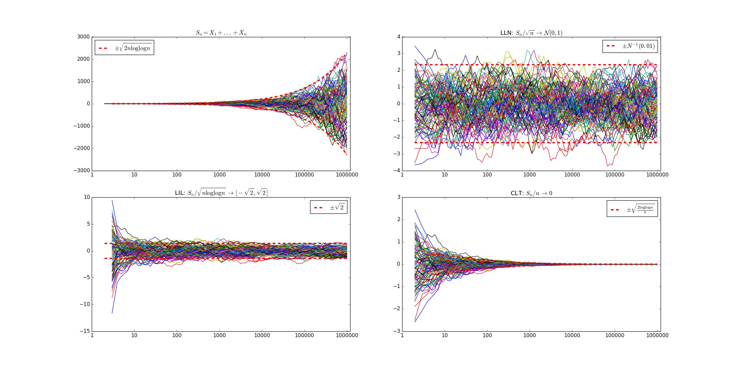
1. If one wants to pursue more deeply the question of why \(n^{1/2}\) is the magic number here for vectors and for functions, and why the variance (square \(L^2\) norm) is the important statistic, one might read about why \(L^2\) is the only \(L^p\) space that can be an inner product space. Because \(2\) is the only number that is its own Holder conjugate. Another valid view is that \(n^{1/2}\) is not the only denominator can appear. There are different “basins of attraction” for random variables, and so there are infinitely many central limit theorems. There are random variables for which \(\frac{X_1 + \dotsb + X_n}{n} \Rightarrow X\), and even for which \(\frac{X_1 + \dotsb + X_n}{1} \Rightarrow X\). But these random variables necessarily have infinite variance. These are called “stable laws”. It’s also enlightening to look at the normal distribution from a calculus of variations standpoint: the normal distribution \(\mathcal{N}(\mu, \sigma^2)\) maximizes the Shannon entropy among distributions with a given mean and variance, and which are absolutely continuous with respect to the Lebesgue measure on \(\mathbb{R}\) (or \(\mathbb{R}^d\), for the multivariate case). This is proven here, for example. ↩