The abracadabra problem and the penalty for self-similarity

Imagine you’re flipping a fair coin over and over, waiting for certain patterns to arrive. Which pattern will take longer on average: HHH, or HTH? Alternately, let a monkey strike typewriter keys at random, and ask whether the words BAAA or AREA will take longer to arrive on average. Or will it be the same? I’ve heard this called the “abracadabra” problem (in Williams’ Probability With Martingales).

The form the answer takes is that there’s a waiting time for a “generic word” of length N, and then you apply a penalty that makes certain words take longer. Can you guess anything about the penalty? What kind of character it might have? It’s counter-intuitive to me.

Answer: In general the waiting time is \((\text{alphabet size})^{\text{length}}\). But then you add a penalty: for any proper terminal subsegment \(S\) of the word which is also an initial segment, you have to add \(A^{\operatorname{length}(S)}\). (You can think of the \(A^{\text{length}}\) term as the penalty for the whole word being a terminal segment which is also an initial segment.)

The penalty term via Kac’s lemma and de Bruijn graphs

One way to look at the problem is with Kac’s lemma, from ergodic theory. (Kac is pronounced “kahts”.) To review the definition of ergodic: suppose \(T: X \to X\) is a measure-preserving transformation on a probability space. \(T\) is called ergodic if for every \(E\) in \(\Sigma\) with \(T^{-1}[E] = E\), either \(\mu(E)=0\) or \(\mu(E)=1\).

(Thinking that \(T[E] = E\) just when \(E\) has measure 0 or 1 may be more intuitive. \(T^{-1}[E] = E\) just when \(\mu(E) = 0\) or \(1\) is stronger. Intuitively, \(T\) “mixes up the whole space”.)

One way ergodic theory hooks up with mainstream probability theory is that you have a Markov chain and \(T\) is the “advance one time step” operator, which is measure-preserving on a stationary distribution, and which is ergodic if the chain is irreducible.

Let’s return to the case we were just talking about, where the monkeys are typing randomly on a keyboard. For convenience, pretend that the sequence of keystrokes the monkeys make extends infinitely far backward into the past and forward into the future. This fiction is more important than it seems at first. One consequence is evident right away: now the chain is already at the stationary distribution, not just converging to it. This is a particularly simple Markov chain where each individual letter arrives completely independently of all letters before it. And we’re just choosing from a uniform distribution on all 26 characters.

We can modify our perspective on the chain so that the state space is not single letters, but sequences of four letters. Now states do not arise independently anymore. Obviously if the 4-letter window currently reads “KDLT”, the only states accessible to me after one step are DLT*. But the Markov assumption still holds. And because it’s a nice chain (irreducible and aperiodic) it has a stationary distribution to which it converges. It’s not hard to believe that that stationary distribution is the uniform distribution on \(\text{letters}^4\). So the shift operator looks like:

And it’s measure-preserving with respect to the uniform distribution: starting with the uniform distribution on \(\text{letters}^4\) and applying \(T\) to our random variable, we are still in the uniform distribution on \(\text{letters}^4\). Because the future is just as random as the past.

Kac’s lemma says: suppose I pick any set \(A \subset X\) of positive measure, and pick some \(x \in A\). Then I start applying \(T\) to \(x\) over and over. The average number of applications of \(T\) before \(T^{(n)}(x)\) ends up back in \(A\) again is \(1/\mu(A)\).

So applying Kac’s lemma to our case, if I pick my set \(A\) to be a singleton, say \(\{'AREA'\}\), then that set has measure \(1/26^4\), and Kac’s lemma informs me that, after it occurs, on average I will have to wait \(26^4\) time periods before it occurs again.

Notice there’s no penalty term here for matching initial/terminal segments. Our original problem was about the waiting time for a word when we start with a blank page, and we claimed that the waiting time is longer when words have matching terminal/initial segments. Kac’s lemma, on the other hand, is talking about the waiting time to get back to a word when it’s already the current word, and that is the same for every word. Developing some intuition for why these should be different is the goal of this post.

A couple examples

Suppose we’re at the word “ABCD”. The quickest we could possibly get is to back to “ABCD” is in four stages, and there is only one possible return path of length four, namely “ABCD -> BCDA -> CDAB -> DABC -> ABCD”. That sequence has probability \(1/26^4\), and so \(1/26^4 \cdot 4\) is the first of the infinitely many terms summed up to give us the expected return time, which Kac’s lemma informs us is \(26^4\).

Now consider “AREA”. It’s different in that it possesses a return path of length three, namely “AREA -> REAR -> EARE -> AREA”. But the expected return time is still the same, \(1/26^4\). So our intuition should be that the paths surrounding “AREA” are more insular than the paths surrounding “ABCD”: it’s slightly harder to get into “AREA” from “the outside” if you’re just wandering around the de Bruijn graph, which balances out the effect of the length-three return path on the average return time. This is the source of the discrepancy between the expected waiting time for the first occurrence and the expected return time.

We can get some intuition for this by thinking about the de Bruijn graph: when a word has matching initial/terminal segments, there are fewer outside paths into it. So if you have “TATA”, one of the \(26^2\) words which are distance 2 away is “TATA” itself, and therefore there are slightly fewer paths in for a “first visit”. And if we think about waiting for the monkeys to type “TATA”, the first four keys the monkeys type have an equal chance of hitting any of the \(26^4\) possibilities, but if we don’t get lucky early, thereafter, there is a subtle bias away from wandering into “TATA”, compared to words which don’t have any proper prefixes equaling suffixes. Because the web of other nodes that have a 2-step path to “TATA” is slightly smaller. Like a little bottleneck in the inward paths.

For another example, let’s go simpler and consider monkeys striking a typewriter with only two keys, and examine the waiting time for binary words of length two.

1. The waiting time for monkeys on a binary typewriter to hit “11” is \(6 = 2^2 + 2^1\), with the \(2^1\) term being the penalty for “11” having a terminal segment (of length 1) matching an initial segment. “00” and “11” have expected waiting time 6, and other words have expected waiting time 4.
2. If we allow the binary keyboard monkeys to extend infinitely back into the past, we are at the uniform stationary distribution on 2-letter words.
3. Therefore, Kac’s lemma says that if the monkeys have just typed “11”, the expected time before they type it again is \(1/\mu(\text{'11'})\) for \(\mu\) the stationary measure, so \(1/(1/4) = 4\).
4. Every word has the same expected waiting time to return to itself. But nodes like “11” have a particularly easy path to return to themselves. So they must be harder to get to from the outside. (Makes sense, they have only one incoming link from a different node, while other nodes have two such links.)

Visual proof of Kac’s lemma

Another way to state Kac’s lemma: Let \(A \subset X\) have positive measure, and define the random variable \(n_A(x)\) to be \(\inf \{n>0 : T^n(x) \in A \}\). Then \(\int_A n_A = 1\). The integral of a function \(f\) over a set \(S\) of measure \(\mu(S)\) can be interpreted as \(\mu(S)\) times the average of \(f\) on \(S\). So here Kac’s lemma is saying that \(\mu(A)\) times the average of \(n_A\) on \(A\) is 1, or the average of \(n_A\) on \(A\) is \(1/\mu(A)\).

Proof: (Taken from Charles Walkden) Every \(x \in X\) will almost surely end up with \(T^n(x)\) in \(A\) eventually (by ergodicity, I claim without proof). So partition up the space like this:

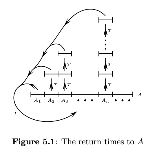
Define

\[A_n \overset{\text{(def)}}{=} A \cap T^{-1}[A]^C \cap \dotsc \cap T^{-(n-1)}[A]^C \cap T^{-n}[A],\]

that is, the set of points in \(A\) which return to \(A\) after exactly \(n\) applications of \(T\). The levels above each \(A_n\) all have the same measure, because \(T\) is measure-preserving. They represent the images \(T^{(i)}A_n\), which are not in \(A\), by definition. Almost every point of \(X\) is in some level above some \(A_n\) by ergodicity. And all those levels above all the \(A_i\) must be disjoint, otherwise they’d violate the definition. So counting \(\sum \mu(A_i) \cdot i\) is the same as counting the measure of almost every point of \(X\), which is 1. In our example, with \(A = \{\text{'TATA'}\}\), we would have \(A_2 = \{\text{'TATA'}\}\) nonempty, with \(\{\text{'ATAT'}\}\) lying over it.

The penalty term via gambling and optional stopping

OK, maybe that was good intuition, but this way will actually let us derive the formula for the penalty term in a generalizable way.

Aside on stopping times

Say I have a Markov chain \(X_k\), and I truncate it with a random stopping time \(T\). In other words, the modified chain \(X_T\) is the one that is \(X_1, X_2, X_3,\) as usual, until time \(T\), and after that \(X_{T + 1} = X_{T + 2} = \dotsb\) forever. \(T\) is supposed to be a rule for stopping, which you can think of as a strategy for when to walk away from the table. (Like for instance, “I’ll stop playing once I either win $50 or lose $20.”)

It confused me a bit at first, how to think of a variable \(T\) which is a “time to stop”. It’s random, but it can depend on \(X_k\) (like the example I just gave, which depended on my winnings at time \(k\)). So what is a stopping time generally? What does it “know”?

The setting for a Markov chain \(X_k\) (or any discrete-time stochastic process) is a filtration \(\mathscr{F}_0 \subset \mathscr{F}_1 \subset \mathscr{F}_2 \subset \dotsb\) of \(\sigma\)-algebras, so that \(X_k\) is \(\mathscr{F}_k\)-measurable for all \(k\) (and therefore \(X_k\) is also \(\mathscr{F}_{k + j}\)-measurable for \(j \geq 0\).) That is, \(\mathscr{F}_k\) knows the value of \(X_k\), but \(\mathscr{F}_k\) might not know the value of \(X_{k + 1}\).

For short, we say “\(X_k\) is adapted to filtration \(\mathscr{F}_k\).” The weird thing about a stopping time is: which of the \(\mathscr{F}_i\) is \(T\) measurable with respect to? All of them? That would mean we already know the value of the stopping time at time 0, which isn’t what we want. (We don’t know at time zero if we’re going to win or lose, or how long either of those things will take.) Maybe \(T\) is measurable only with respect to the union, \(\mathscr{F}_\infty\)? That’s not really enough to assume, because that means at a given time \(k\), the \(\mathscr{F}_k\) doesn’t necessarily know whether I stopped yet or not. I should at least know if I’ve stopped. The right way to put it is that \(T\) is not necessarily measurable with respect to any \(\mathscr{F}_i\), but the event \(\{T = k \}\) (and its complement) are in \(\mathscr{F}_k\) for all \(k\). At each time, we know if we’ve stopped or not, but not necessarily before. So the event \(\{T = k \}\) can depend on the value of \(X_k\), or on other stuff that we know about at time \(k\).

Aside on martingales

OK, a chain with a stopping time. In fact, we don’t actually want a Markov chain for the optional stopping theorem; we want a chain that is a martingale, which models a fair game. Specifically, a chain \(M_k\), adapted to a filtration \(\mathscr{F}_k\), such that \(\mathbb{E}(M_k - M_{k -1}\mid \mathscr{F}_{k -1}) = 0\) for all \(k\). So at time \(k -1\), my expected gain in the next stage is zero.

It is also then true that just the plain old expectation \(\mathbb{E}(M_k - M_{k -1}) = 0\). But that’s a weaker statement. (That’s like taking the expectation at time zero, or conditional on level \(\mathscr{F}_0\) of the filtration.) The stricter, martingale condition says: even with all the extra information I have gathered from time 0 to time \(k - 1\), my expected gain \(M_k - M_{k-1}\) is still zero. In particular, we can telescope:

\(\mathbb{E}M_k = \mathbb{E}(M_0 + (M_1 - M_0) + (M_2 - M_1) + \dotsb + (M_k - M_{k-1})) = E(M_0)\),

because \(\mathbb{E}(M_k - M_{k-1})=0\) for all \(k\).

When people think of a martingale, they often imagine it with increments \(M_k - M_{k - 1}\) which are all independent (with mean zero). For instance, \(M_n\) being the cumulative sum or average of i.i.d. mean-zero random variables.

But that’s way too restricted a case to be representative of a martingale. Every chain \(X_k\), no matter how weird or dependent the increments are, can be seen as a martingale, after a minor modification: just subtract the conditional mean at each step.

\(M_k \overset{\text{(def)}}{=} X_k - \mathbb{E}(X_k \mid \mathscr{F}_{k - 1})\) is a martingale.

It’s akin to how you can write a random variable \(X\) as a mean-zero random variable plus a deterministic term. \(X = (X - \mathbb{E}X) + \mathbb{E}X\). Except now you’re splitting a chain into two chains: \(X_k = M_k + \mathbb{E}(X_k \mid \mathscr{F}_{k - 1})\). That latter term isn’t deterministic like the mean \(\mathbb{E}X\) is, but it is predictable. In other words, it’s something taking place at step \(k\), whose value you already know at step \(k - 1\). (That is to say, unlike \(X_k\) or \(M_k\), the variable \(\mathbb{E}(X_k \mid \mathscr{F}_{k - 1})\) is \(\mathscr{F}_{k - 1}\)-measurable.) You don’t know the value of \(\mathbb{E}(X_k \mid \mathscr{F}_{k - 1})\) at time zero, but at least you know its value one step before it “happens”.

\(\mathbb{E}(X_k \mid \mathscr{F}_{k - 1})\) is called the “drift” term. Any reasonable stochastic process is (martingale + predictable drift) (Doob decomposition theorem). I like that term “drift”. Like we’re carving out the randomness at each step into its essential parts, and the part of it that’s less interesting is just the momentum from the previous step. The part I could already predict.

Back to the point

OK, so martingales and stopping times. The optional stopping theorem says very simply that a stopped martingale is a martingale. So given a martingale \(M_k\) and a stopping time \(T\), the chain \(M_T\) is also a martingale. In particular, \(\mathbb{E}(M_T) = \mathbb{E}(M_0)\), like for any martingale. In other words, no clever strategy I can form for stopping my play is ever going to let me beat the house on average. My expectation on my play will remain \(\mathbb{E}(M_0)\), for any stopping strategy I choose. (Nor can I lose money on average on a fair game if concoct a devious plan to do myself dirty.)

Now, how does this relate to the abracadabra problem? Pretend I am the house, and gamblers are coming in and placing fair bets on the monkey who is hitting random keys on the typewriter. We can imagine all kinds of fair bets, but for convenience let’s confine ourselves to bets which are decided after a single round. So a gambler might take 1:1 odds on the ASCII code of the letter that comes up being even. Or they might take 25:1 odds on a certain letter coming up, you get the point. Define the martingale \(M_k\) to be how much I (the house) have profited or lost at time \(k\). I’m going to stop my martingale when “ABRACADABRA” hits. So \(M_T\), my stopped martingale, has \(\mathbb{E}(M_T) = \mathbb{E}(M_0) = 0\) by the optional stopping theorem.

The gamblers coming in can be playing any strategy–as long as each round has expectation zero for each of them, my profits/losses remain a martingale. In particular, this universe can contain very specific gamblers whose behavior casts light on this problem. I sit the monkey down at the typewriter, and I invite gamblers in. At every time period, a new gambler comes in and places a $1 bet on “A”. Since it is a fair game, she gets $26 if she wins. (Or $25 of my money and $1 of hers back, if you like. But it’s more convenient to treat the $1 as mine as soon as she gives it to me.)

If the gambler wins her “A” bet, she doubles down on “B”, betting \(\$26\) to win \(\$26^2\). If she wins that, she doubles down on “R”, and so on, until “ABRACADABRA” hits. (Which is when I end the game, recall.) Recall also that a new gambler arrives at every stage, regardless of whether the previous person is still playing or not. So there are sometimes multiple people playing at once.

Of course many, many gamblers are likely to lose before “ABRACADABRA” comes. I will have made $1 from each of their losses. My expected profits \(\mathbb{E}M_T\) are zero, as I mentioned. They are also equal to my expected gains minus my expected losses. \(\mathbb{E}M_T = \mathbb{E}(\text{gains} - \text{losses})\). My gains are exactly $1 for each time period that has gone by. (One new gambler showed up every period and staked $1.) So my expected gains are exactly the amount of time that goes by before I end the game. (Or at least the way I’m counting things, they are.)

But my losses are deterministic! When “ABRACADABRA” eventually hits (I claim it will, with probability 1), I will be down some serious money. In fact, there will be three gamblers playing when that happens, all of whom will get money from me. (Because of the terminal segments that match initial segments.) The amount I will lose is

\[26^{\text{(length of 'ABRACADABRA')}} + 26^{\text{(length of 'ABRA')}} + 26^{\text{(length of 'A')}}\]

Therefore that is exactly my expected profits, and that is exactly the expected time that goes by before it hits.